This writeup is based on a project I performed for a major national laboratory. I cannot get into the details, so instead, here I cover the methods and general scope of the project: combining input distributions from several experiments into a consensus model. This consensus model represents the combined understanding of all relevant experiments.

Averaging Probability Distributions

To begin with we examine the difference between arithmetic or probability averaging and Wasserstein or quantile averaging. Probability distributions, just like numbers, vectors, matrices, and other quantitative objects, may be averaged together. However, distributions have more ‘pieces’ in their definition and construction than simple numbers and arrays, so averaging them is also more complicated.

Two primary methods for averaging probability distributions are probability averaging and quantile averaging. The images below depict each case. Our averaging inputs are two Gaussian distributions with equal variance but different means. These are visualized in light yellow in each graph. The red distribution is the average; the left image depicts the probability average and the right image the quantile average.

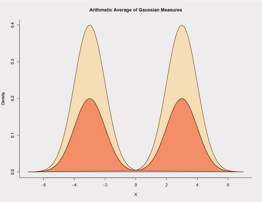
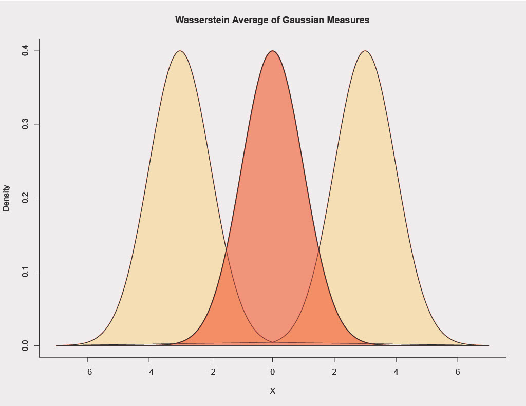
We may prefer one or the other, depending on the application of interest. In a nutshell, probability averaging is useful when input probability distributions represent different portions of the same phenomenon, and quantile averaging makes the most sense when input probability distributions are modeling the same portion of the same phenomenon. In the image above, assume each Gaussian input is a distribution from a sensor measuring a feature, something like equipment temperature. The following two scenarios apply to probability and quantile averaging respectively.

Scenario 1: Imagine one sensor is a daytime temperature sensor and the other a nighttime sensor. Then here we prefer the probability average, as each sensor is measuring a separate part of the full distribution, i.e. the full day-night distribution is truly bimodal, and each sensor catches one mode.

Scenario 2: Imagine each sensor runs all day, and is on average unbiased, but there is some noise in the mean value of each distribution. In this case we prefer quantile averaging as each sensor is measuring the same phenomenon but has its own noise, i.e. the full distribution is truly unimodal.

To read a bit more about probability vs quantile averaging, see the following paper (Schepen & Wang, 2015).

From Probability Distances to Probability Averaging

Closely related to the idea of averaging is the idea of distance. An average cannot be taken without some notion of distance.

The Fisher-Rao and the Wasserstein metrics are two statistical distances between probability distributions closely related to the idea of probability and quantile averaging. The Wasserstein metric may be used to obtain barycenters; in 1D this equivalent to quantile averaging, and it generalizes the idea of quantile averaging to higher dimensions, as quantiles do not exist beyond 1D. Probability averaging minimizes the Kullback-Liebler divergence, a quantity closely related to the definition of the Fisher-Rao distance, which may also be used to construct barycenters. To see a somewhat technical comparison of Wasserstein and Fisher-Rao distances in constructing barycenters of multivariate normal distributions in the space of radar signal processing, seee the following (Barbaresco 2011).

The mathematics behind these ideas is bit advanced. However, a recent paper (Marti et al 2016) compared and contrasted the uses of each distance in a multidimensional setting where distributions exhibit dependencies. In this setting, the authors found that Wasserstein distance-based methods preserve geometric information in a more consistent manner than Fisher-Rao and other Kullback-Liebler-based methods. There are deep mathematical reasons for this; however the following example from their paper serves a succinct, intuitive example. Consider the following three 2D normal distributions. Each is a standard bivariate normal but with correlations of .5, .99. and .9999 respectively.

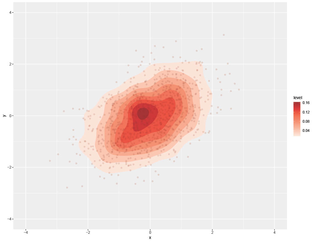
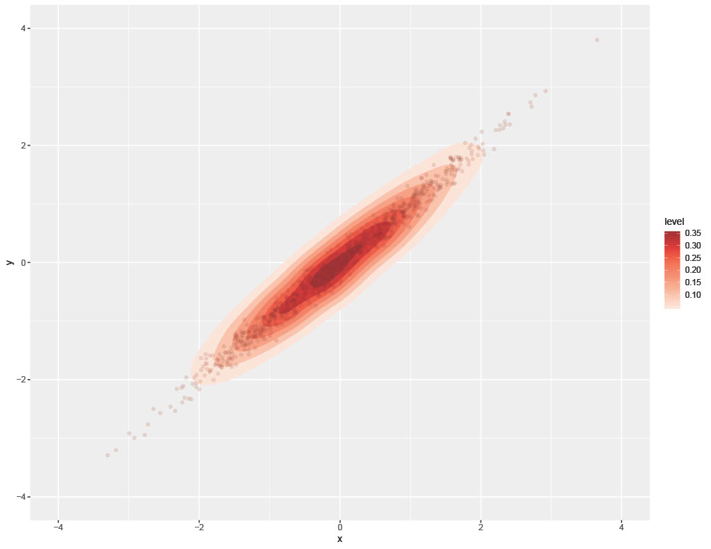
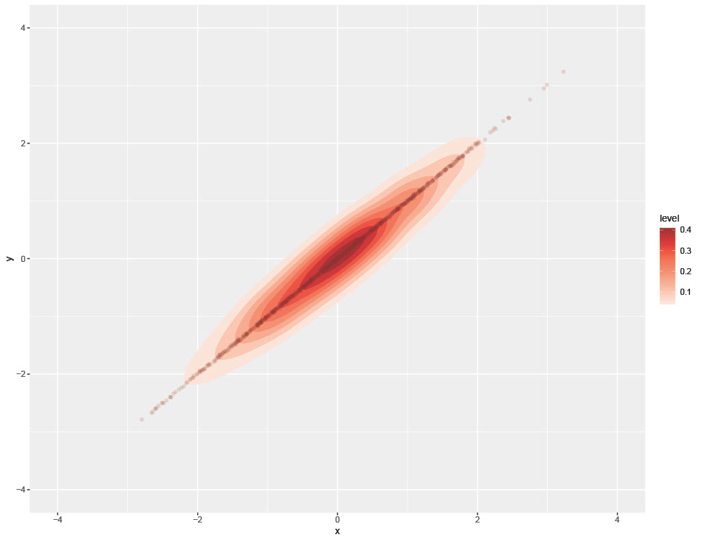
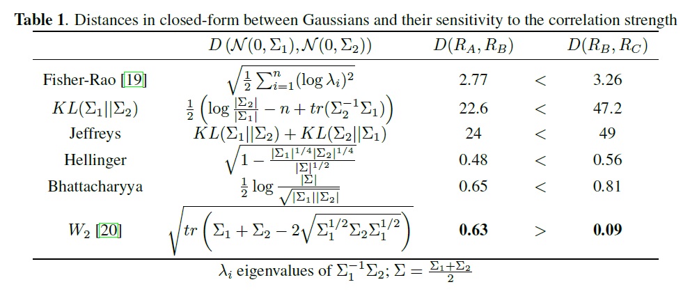
Intuitively, by looking at these images, we can readily see that 99% and 99.99% correlation distributions should probably be closer distance-wise than 50% and 99%. Nonetheless, the authors find that Fisher-Rao and several other Kullback-Leibler-based distances all rank 99% correlation as closer to 50% than to 99.99%. Only the Wasserstein distance respects our intuition that 99% and 99.99% correlation bivariate Gaussians should be closer. This captured in the following table from their paper (Table 1, pg 4).

Barycenters and Consensus Modeling

For this research project, I was tasked with designing a consensus modeling framework for combining inferences from several related experiments. Previously, this lab relied on consensus Monte Carlo (CMC) for consensus modeling. The CMC algorithm was published in (Scott et al 2016) by a Google research team collaborating with several university professors as way of handling big data. Essentially data is split up (due to intractable size) and processed on different computers. The outputs from these machines are then combined in a systematic way to give a ‘consensus’ picture across the entire dataset. A basic overview of the method is as follows:

1. split data set into groups called “shards” and assign each shard to a worker machine
2. each machine performs Monte Carlo simulation to fit a posterior distribution for parameters
3. output parameters from each shard are combined with a weighted average

In the setting of normal distributions, this task is straightforward: a simple formula for the weights is known and CMC has strong guarantees. The method is somewhat robust to departures from this normality assumption. In general, if the data set is large enough, and we have sufficient data in each shard, the weights can safely be assumed to equal across all shards. However, if the data is this uniform across different shards, then it is likely that the data distribution is relatively simple and does not warrant big data and heavy computation to be characterized. Hence consensus modeling is most useful in those cases where data is complex enough to warrant big data.

In our original experimental setting there were a few issues with implementing CMC. All experimental distributions were not necessarily Gaussian. In fact, each experiment collected data on different portion of the full distribution. The experimental distributions of interest were bivariate and exhibited various patterns of dependency. CMC does not preserve and integrate dependency in a meaningful way in all settings.

Here Wasserstein-based combination methods were implemented and assessed for consensus modeling as a more robust method than CMC. Two Wasserstein-based algorithms were deployed for this consensus modeling problem:

• Wasserstein scalable posteriors (WASP) (Srivastava et al 2015), (Srivastava et al 2018)
• fixed-point Wasserstein barycenters (FPW) (Álvarez-Esteban et al 2016)

The WASP method is a linear programming approach that approximates the full Wasserstein barycenter problem. A full Wasserstein barycenter requires restrictively massive computation for this type of problem. The WASP method offered a strong approximation that converges to the true Wasserstein barycenter as the limit of samples grows larger and larger. Its strength: it is highly flexible; different experiments can have virtually any distribution and still be combined in a meaningful way.

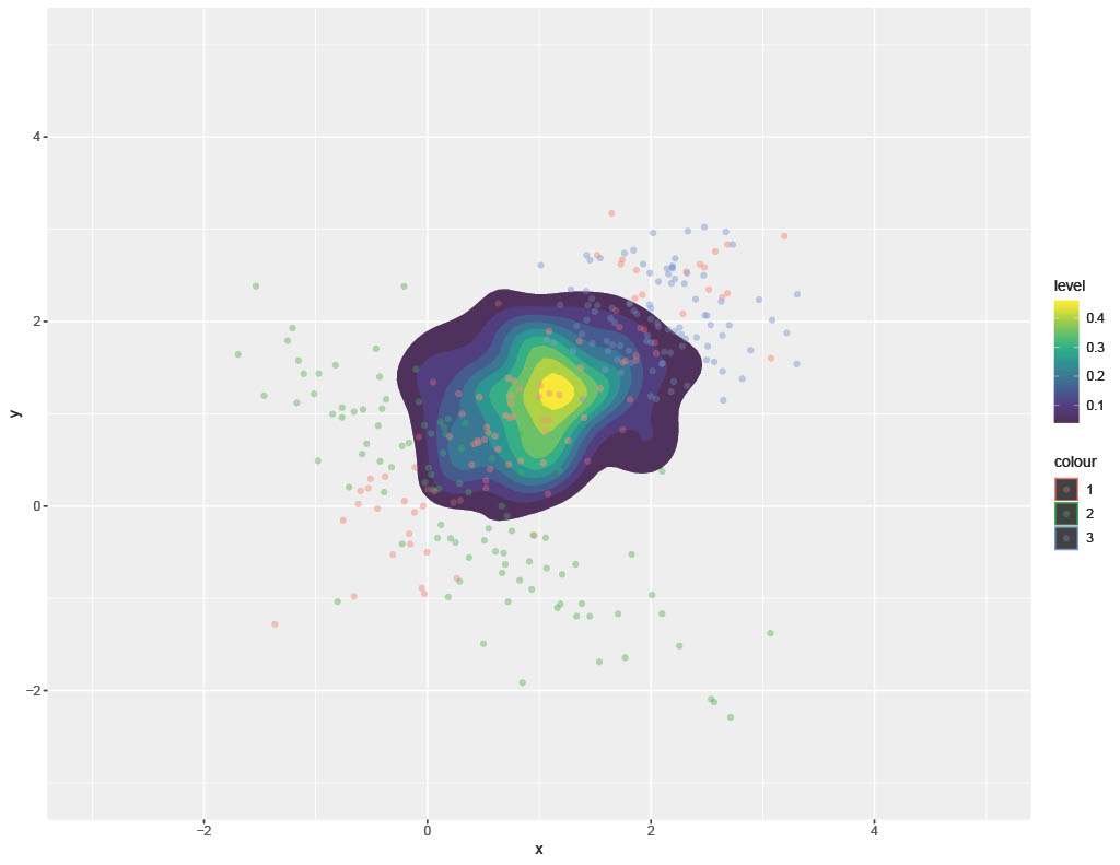
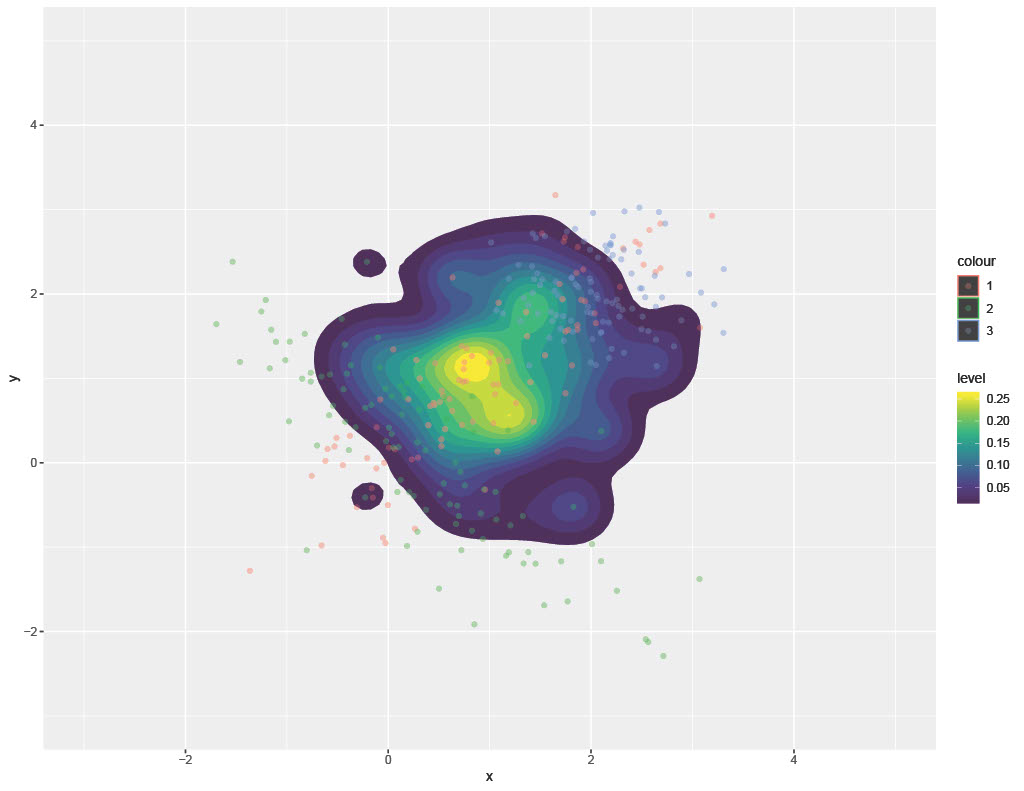
This method was found to be more effective at preserving and integrating dependency information across different experimental distributions. The following images show a comparison of CMC and WASP methods for combining several, disparate bivariate distributions. Not that CMC wants to squish everything into a ‘rounded’ spherical patterns whereas the WASP algorithm is more effective and contouring the consensus model in a manner that integrates dependency information from individual input distributions. The colored, faded points below are the input samples (from different distributions) and the colored region represents the consensus probability density.

One major challenge with the WASP method is its limits in scalability. Ironically, while WASP is more flexible than CMC, hence far more appropriate for complex consensus modeling problems, it is computationally not as efficient as CMC. Here the FPW method was deployed as an alternative that is far more scalable than WASP (and even CMC in many settings) at the cost of some loss of flexibility.

The FPW algorithm boils down to a set of matrix and arithmetic operations until convergence. It is more limited than WASP in that the distributions must come from the same location-scale family. The algorithm tends to converge quickly and scales with the number of parameters in the scale matrix. Hence, when sample sizes are large but dimensions are relatively low, the FPW approach has a far more favorable computational scaling than either CMC or WASP. In the case of this lab’s experiments, distributions were not necessarily Gaussian but in the same location-scale family, sample sizes were very large, but parameters of interest were few.